DLA(Diffusion Limited Aggregation) and DBM(The Dielectric Breakdown Model)

If you want to view the source code, you can search for them in my GitHub repository.

1.Abstract

DLA(Diffusion Limited Aggregation) and DBM(The Dielectric Breakdown Model) are two commonly used non-equilibrium growth models. DLA is a classic model for non-equilibrium growth, used to study natural phenomena such as crystal growth, fluid dynamics, and dust aggregation. On the other hand, DBM is a model for dielectric breakdown phenomena, used to predict breakdown behavior in materials by considering physical processes such as the density evolution of ionized electrons and electron holes. Despite being applied in different fields, both models share the common feature of non-equilibrium growth, where the evolution of physical processes does not satisfy thermodynamic equilibrium conditions.

In this article ,I simulated 2D DLA and DBM patterns, and discussed image’s fractal and dimensional features.

Keywords : Random walking,growth model, Laplace Equation, fractals and fractal dimensions

2.Method

2.1 DLA

The DLA model is one of the classic models for describing non-equilibrium growth, and its basic idea is that particles with random motion deposit on an adsorption center to form a dense shell in an initial state. New particles diffuse and move along the surface of the shell, and if they collide with a certain point of the original shell, they will stop and be adsorbed, continuing to form the next layer of the shell. The DLA model is commonly used to study non-equilibrium growth phenomena in nature, such as crystal growth, fluid dynamics, and dust aggregation.

Simulation Rules

A 2D square lattice is taken, and a particle is placed at the center of the lattice as the seed for growth. Another particle is released from a circular boundary far enough from the origin of the lattice and allowed to perform a random walk. The particle will eventually collide with the nearest neighbor position of the seed, at which point the particle will stick to the seed and stop moving. If the particle reaches the boundary of the lattice, it is considered a useless trajectory and discarded, and a new particle is generated. Therefore, useful particles that stick to the seed form a growing aggregate cluster.

Definitions:

• The maximum distance of the current aggregate cluster is d.
• The cluster radius is $r=\max({20, d})$.
• The edge length of the 2D square matrix is $N$.
• The particle stickiness is $stickness \in (0,1)$.
• The radius of the generating circle is $R=2r$.

Algorithm:

1. Randomly generate a particle, $x$.
   • If $R<N/2$, generate a particle randomly on a circle with radius $R$.
   • Otherwise, generate a particle randomly on the boundary of the square lattice.
2. Let particle $x$ perform a random walk and check if there are any aggregate particles in the eight surrounding points.
   • If the particle collides with the boundary of the lattice, return to step 1 and generate a new particle.
   • If there are aggregate particles nearby, determine whether to join the cluster or continue to perform a random walk based on the stickiness of $x$.
3. When the particle joins the cluster, update the cluster radius, $r$.
4. Return to step 1, or end the program when the cluster is large enough.

2.2 DBM

The DBM model is a model that describes the dielectric breakdown phenomenon. When an external electric field reaches a certain strength in a dielectric material, the electrons inside the material are subjected to a strong enough electric field force and collide with ionized electrons, resulting in local breakdown. The DBM model establishes the evolution equation of the ionized electron and electron hole densities in the dielectric material by considering physical processes such as free electrons, positive ions, and electron holes in the material, which predicts the breakdown behavior in the material. The DBM model is commonly used in the design of electrical equipment, optoelectronic devices, semiconductor materials, and so on.

Simulation Rules

The process described by this model involves a constant potential $\phi_0$ at the central point of a dielectric material (insulator), which continuously breaks down the surrounding medium, forming a growing conductor.

The growth rate $v$ of breakdown in the medium is a function of the gradient of potential $\phi$, i.e., $v=f(\nabla_n\phi)$, where $n$ is normal to the interface. The potential throughout the medium follows Laplace’s equation, and the boundary conditions are that the potential is $\phi_0$ on the occupied grid and 0 at a distance. The growth mode is to occupy an empty grid on the boundary with a probability equal to the growth rate. Mathematically, this can be described as: \(Growth Rate::v_{i,j}=n|\phi_0-\phi_{i,j}|^{\eta}\tag{1}\)

The probability is summed over all unoccupied grids on the boundary, and a grid is selected for occupation based on this probability. After occupying a new grid, the boundary conditions change, and the potential distribution, growth rate, and selection probability need to be recalculated.

Definitions

• Grid state: EMPTY represents a free point, CANDIDATE represents a candidate point, and FILLED represents a grown point.
• Particle set _particle_set: stores a set of generated points, all of which have the state FILLED.
• Candidate set _candidate_set: stores a set of candidate points to be grown, all of which have the state CANDIDATE.

Algorithm

1. Using formula (1) and (2), randomly select a candidate point x from _candidate_set based on its growth rate.
2. Add the candidate point x to _particle_set, change its state from CANDIDATE to FILLED, and set its potential to $\phi_0$.
3. Add all surrounding EMPTY points of x to _candidate_set, changing their state from EMPTY to CANDIDATE.
4. Remove x from _candidate_set.
5. Recalculate the potential of particles in _candidate_set based on Laplace’s equation and the new boundary conditions.
6. Go back to step 1, or terminate the program when the cluster is large enough.

Note: In actual code implementation, it is not necessary to label points with states. The state can be determined based on whether a point is in _particle_set or _candidate_set.

Numerical Solution Method for Laplace’s Equation:

The Laplace equation can be expressed as

For numerical solution, it can be written as \(\phi_{i,j}=(\phi_{i-1,j}+\phi_{i+1,j}+\phi_{i,j-1}+\phi_{i,j+1})/4\) In reality, the potential values of the surrounding points are not known, only the potential values on the boundaries are known. Therefore, particles at position (i, j) are allowed to randomly walk until they encounter the boundary, at which point the potential value on the boundary, denoted as $f(x,y)$, is recorded. After multiple random walks, the average potential value is taken as the potential value at point (i, j): \(\left<\phi_{i,j}\right>=\frac1N\sum_n^N f_n(x,y)\)

2.3 DBM_FAST

Background

For actual dielectric breakdown models, the main bottleneck of the algorithm is to re-calculate the potential size of all candidate points after each iteration. When the boundary range N is large enough to grow n points, the time complexity required is $O(n*N^3)$ 1. For a grid point with a side length of $N=300$, the time will be very slow, and it takes about 18 minutes to grow n=300 points.

Therefore, based on the idea of a paper about fast Laplace growth simulation 1, I propose the following improvements.

Idea

Each “grown” point is insulated, that is, the charge is not redistributed but fixed at the lattice point. For the potential of candidate points, it is a linear superposition of the electric potential of these FILLED growth points.

Consider that the center potential of the boundary is 1 and the potential at infinity is 0. Then, each point charge can be treated as a positive charge, and the potential is \(\phi(r)=\frac{R_1}{r}\) where the length of each small lattice point is $h$, and the radius of the point charge is $R_1=h/2$.

Therefore, for the CANDIDATE point $i$, its potential is the superposition of the electric charge $j$ of all FILLED points: \(\phi_i=\sum_{j=1}^n\frac{R_1}{r_{i,j}}\tag{3}\) The growth rate should also be correspondingly corrected. Let the maximum potential of the candidate be $\phi_{max}$, and the minimum potential be $\phi_{min}$: \(v_i = \left(\frac{\phi_{max}-\phi}{\phi_{max}-\phi_{min}}\right)^{\eta}\tag{4}\) The reason why it can be accelerated is that each time it is iterated, the previous potential can be used for iteration, that is: \(v_i = \left(\frac{\phi_{max}-\phi}{\phi_{max}-\phi_{min}}\right)^{\eta}\tag{4}\) $r_{t+1}$ is the distance between the new position of the FILLED point and each CANDIDATE point.

Algorithm

1. According to formula (4), the growth rate of the candidate point is a probability. After normalization, randomly select a candidate point x from the _candidate_set.
2. Add candidate point x to _particle_set, and its state changes from CANDIDATE to FILLED.
3. Remove x from _candidate_set.
4. Iterate the potential in _candidate_set according to formula (5).
5. Add EMPTY points around x to _candidate_set, change the state from EMPTY to CANDIDATE, and calculate the potential of the new candidate point according to formula (3). In one iteration, no more than 5 points like this.
6. Return to step 1; or when the cluster is large enough, the program ends.

2.4 Code Framework

Due to the need for efficiency in the code involving a large number of operations to check whether points are in a set, we have chosen set as the primary data structure. Its operations of searching with in, adding with add, and removing with remove are all with a time complexity of $0(1)$.

Since the three growth models have similar ideas, a class inheritance framework is designed.

Figure 1:Code Framework

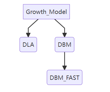
The lower-level classes inherit the interface of the upper-level classes, reducing redundant code.

2.5 Fractal and Dimensional Features

Sandbox Method

Using the Sandbox method to calculate the fractal digits, the formula is

N is the number of pixels in the square box, r is the side length of the box, and C is other constants. The statistical process is shown in the figure below

Figure 2: Sandbox Method

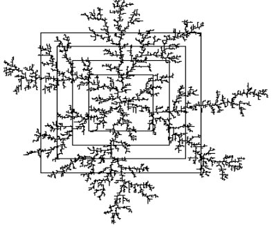
Increase the side length of the box according to the power of $\sqrt 2$, count the number of internal points, and get a logarithmic coordinate graph, and calculate the slope to be the number of fractal digits D

Density-Density Correlation Function Method

The density-density correlation function of fractal patterns in the plane is defined as follows:

where $\rho(r’)$ is the density function of the pattern, which is 1 at the position of the pattern and 0 elsewhere; N is the total number of pixels. The geometric meaning of C(r) is the ratio of the number of overlapping pixels between the original pattern and the pattern translated by r to the total number of pixels, which represents the probability of finding another pixel at a distance r. In actual calculations, the average is taken over N different values of r’, as well as over different directions and lengths of r with the same length.

In the special case where r’ is fixed and taken as the center of the pattern (i.e., r’ = 0), we have:

To determine the fractal dimension, we need to count the number of overlapping pixels within a circle with radius increasing by a power of $\sqrt 2$, plot the results on a logarithmic scale, and obtain the slope $\alpha$.

When integrating C(r) within the turning radius R, the integral value is proportional to the total number of pixels in the pattern when R is large enough.

“dim” refers to the Euclidean dimension of the space, which is 2 in this figure; “D” refers to the fractal dimension.

3. Experiment

3.1 DLA

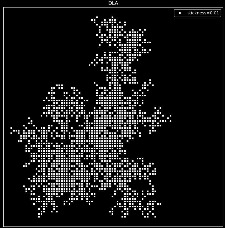
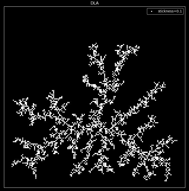
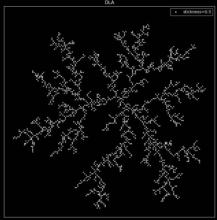
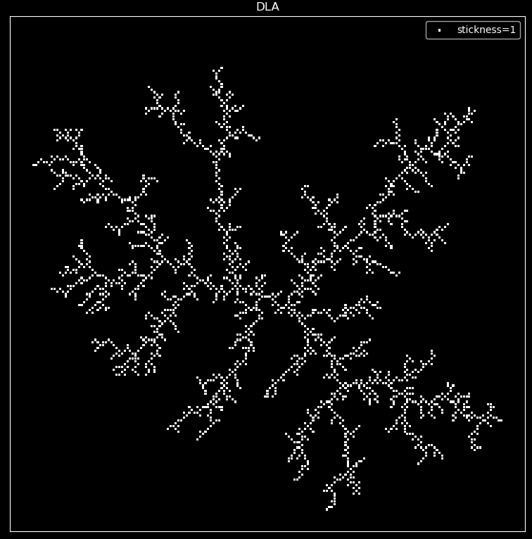
As shown in the following figure, DLA models were considered with viscosities of 0.01, 0.1, 0.5, and 1, respectively, and 3000 points were grown.

Figure 3. Comparison of DLA with different stickiness values (3000 points).

DLA Analysis：

As shown in the figure, as the viscosity increases, the image of DLA growth becomes increasingly sparse. When the viscosity is 1, particles are likely to collide with an external dendrite before entering a trench, resulting in a shielding effect and preventing particles from entering the trench. This structure reflects the characteristics of the growth process, where growth occurs faster at the tips, leading to the formation of branches that extend outward, and slower in flatter areas, resulting in a loose structure with gaps in the trenches. This morphology only appears when particles adhere to the cluster without any preferred direction.

3.2 DBM

As shown in the following figure, DBM models were considered with eta values of 0, 3, 6, and 10, respectively, and only 300 points were grown due to limited code efficiency.

Figure 4: Comparison of DBM with different values of eta (300 points).

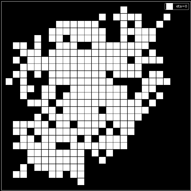
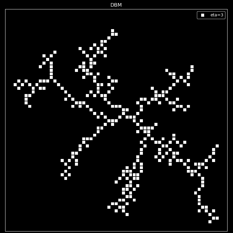
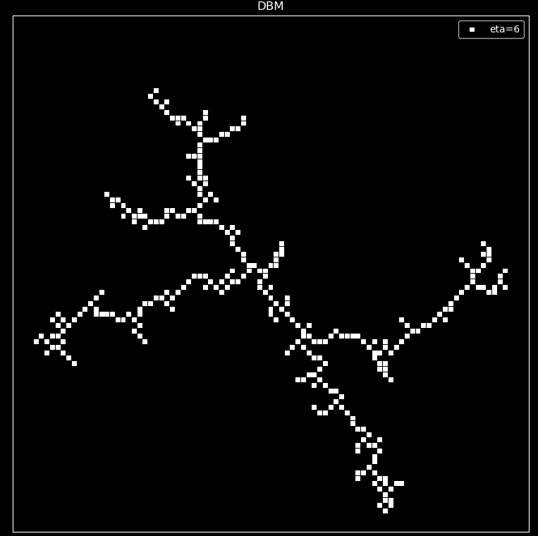
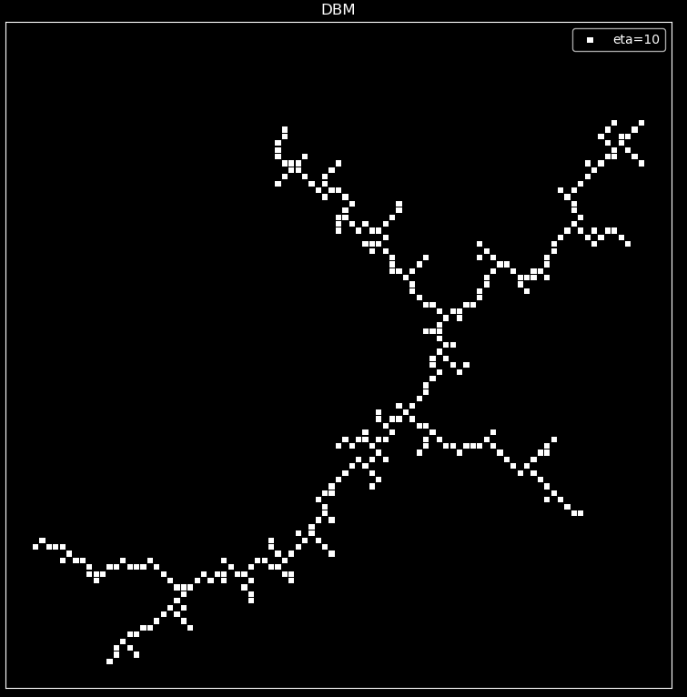
Analysis of DBM:

From the images, it can be observed that as $\eta$ increases and the growth rate \(v_ {i,j}=n|\phi_0-\phi_ {i,j}|^{\eta}\) chooses branches based on probability, the number of branches gradually decreases, and the image converges from a two-dimensional uniform plane to a one-dimensional image, just like from a spherical lightning to a linear lightning.

This phenomenon can be easily explained by analysis. As $\eta$ increases, for larger potential energy gradients \(|\phi_0-\phi_{i,j}|\) their weight becomes more prominent, leading to a greater probability of choosing the direction with a greater change in gradient. Therefore, it is easier to present a linear image with fewer branches.

3.3 DBM_FAST

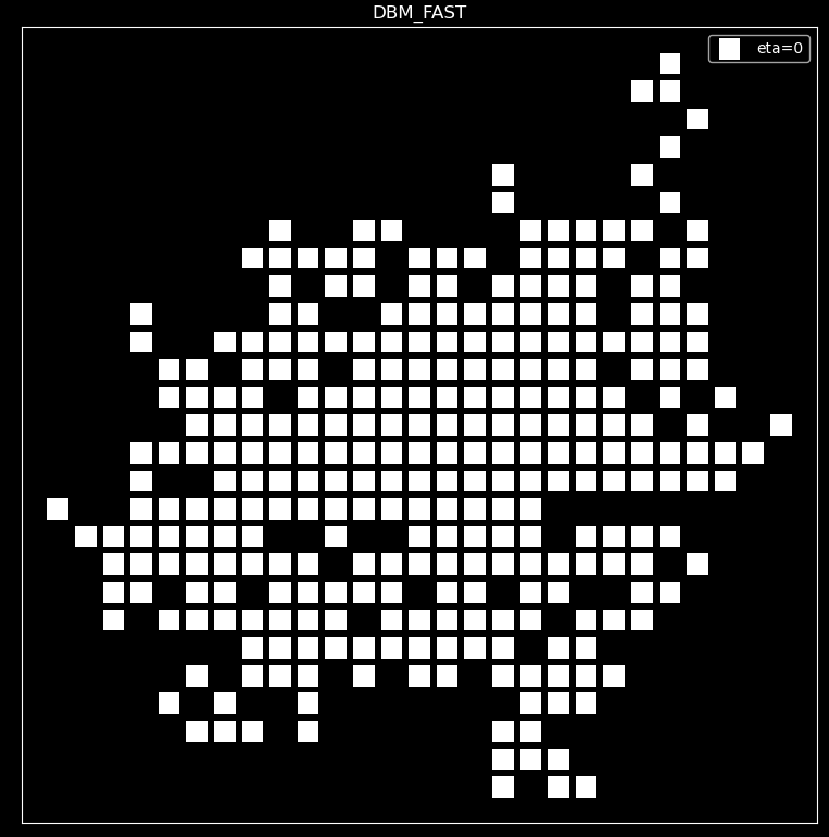
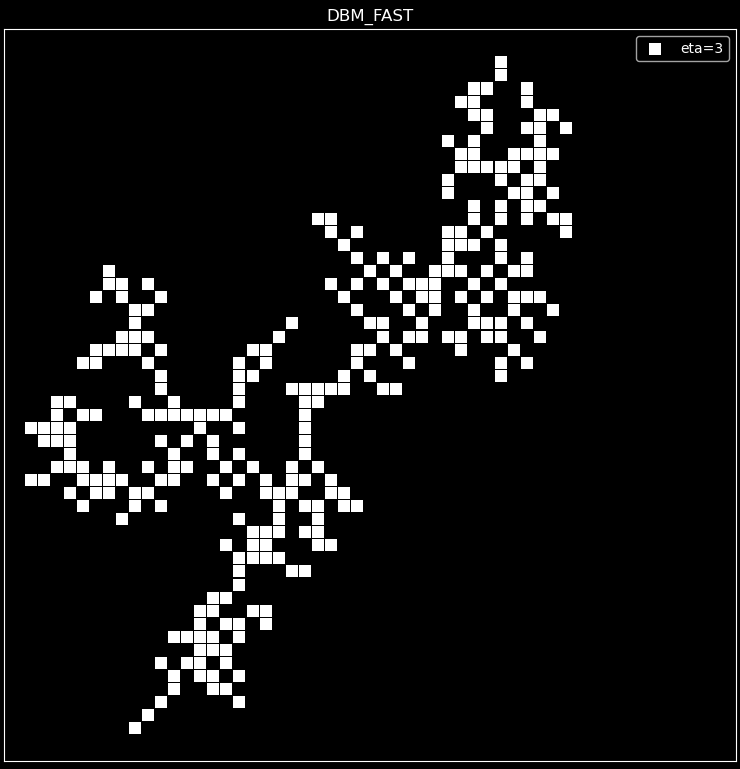
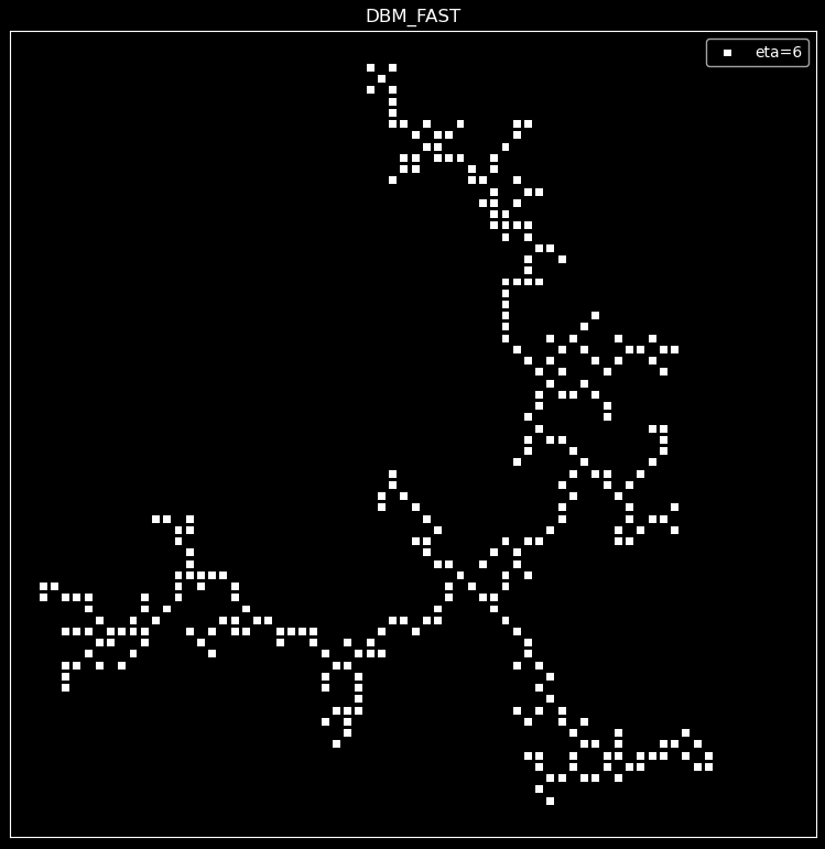
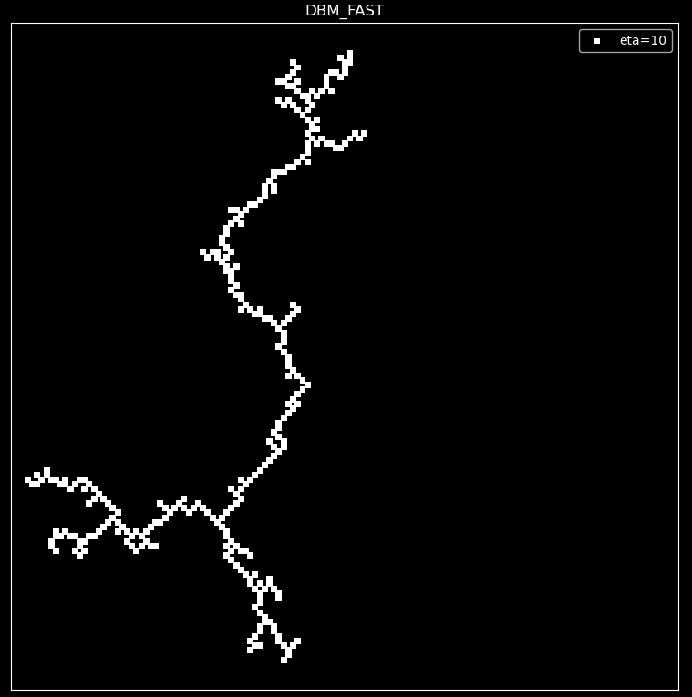
After improving the algorithm, DBM models with $\eta$ values of 0, 3, 6, and 10 were obtained, and 3000 points were grown to produce the following images.

Figure 5: Comparison of DBM FAST algorithm with different eta values (3000 points).

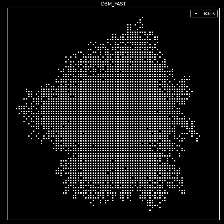
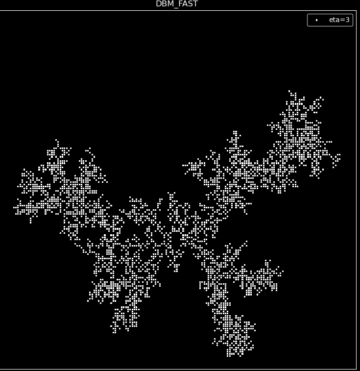
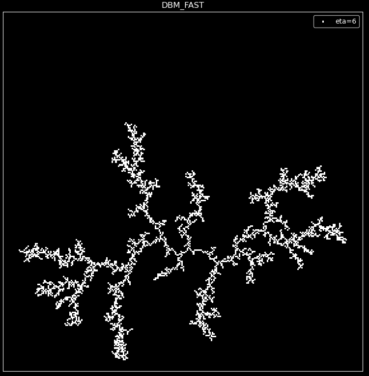
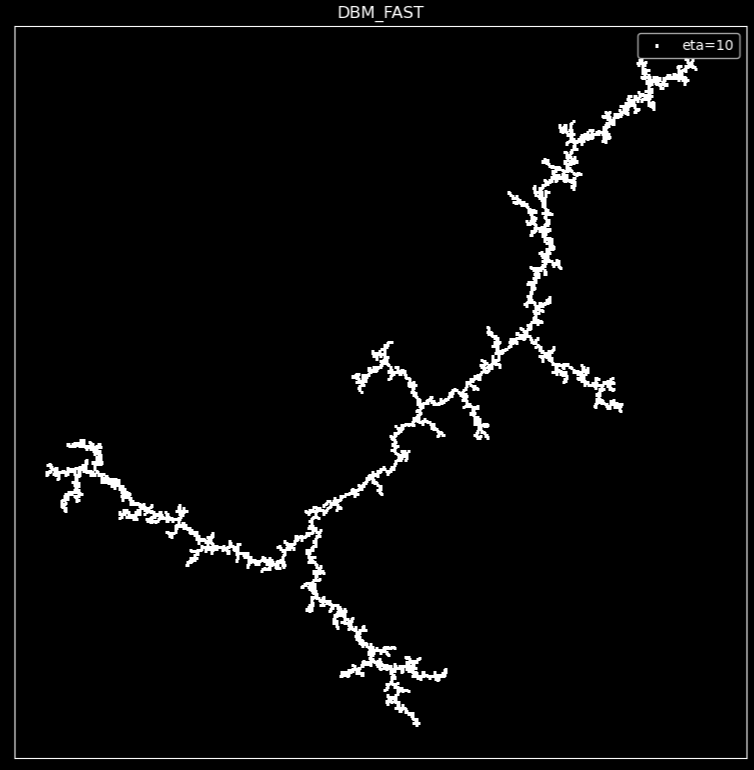
DBM FAST Analysis:

As can be seen from the images, with the increase of $\eta$, the image also gradually converges from a two-dimensional plane to a one-dimensional line, consistent with the trend of DBM. This indicates that our improved algorithm has not changed the essential difference of the image and greatly accelerated the speed of the algorithm.

Comparison with DBM

The following image shows the DBM FAST algorithm with 300 points. They can be better compared with the DBM images(Figure 4).

Figure 6: Comparison of DBM FAST algorithm with different eta values (300 points).

Compared to the DBM image (Figure 4), the two are almost identical.

And the computation time has been significantly reduced.

Figure7: Time Comparison

Almost 1000 times faster.

Compared with DLA

Under certain parameter selections, both exhibit tree-like growth.

It can be seen that the DLA algorithm always maintains a larger number of branches and does not gradually converge to one dimension with changes in parameters. The DBM algorithm, as $\eta$ changes, will make the correlation between points more obvious, converging to one dimension and no longer exhibiting branching phenomena.

3.4 Fractal and Dimensional Features Result

Sandbox Method

​ The experimental results are shown in the following figure

Figure 8: Sandbox Result

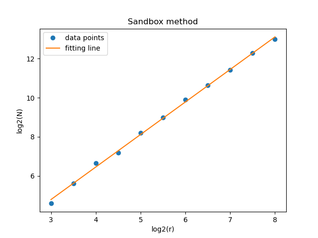
The experimentally computed slope of the image is \(D_1=1.6666788360254807\) which is the fractal dimension.

The fractal dimension result is in the range of 1.6 to 1.7, which is in good agreement with the theory.

2.3 Density-Density Correlation Function Method

The experimental result is shown in the following figure.

Figure 9: Density Result

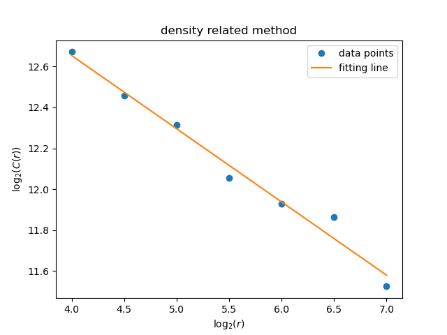
​ The slope of the image and the fractal dimension are： \(k=-\alpha = -0.35808654164728 \\D_2=d-\alpha=1.64191345835272\) ​ The fractal dimension result is in the range of 1.6 to 1.7, which is in good agreement with the theory.

4. Summary

• In this experiment, DLA and DBM models were compared and their differences were analyzed.

• A method to accelerate the Laplace numerical algorithm was proposed and its effectiveness was verified through experiments.

• During the experiment, a good data structure pattern, “set”, was adopted to improve the program speed.

• The dimension of DLA was calculated using the sandbox method and the density-density correlation function method. The dimensions obtained by the two methods were both within the range of 1.6 to 1.7, which is close to the theoretical value

5. Reference

[1] laplacian_large