Using Monte Carlo methods to solve the rendering equation for implementing ray-traced global illumination.

If you want to view the source code, you can search for them in my GitHub repository.

1. Abstract

This article mainly introduces the use of Monte Carlo methods to solve the rendering equation. The rendering equation is decomposed into direct and indirect lighting, and Monte Carlo importance sampling is used for direct lighting, with the Alias algorithm used to accelerate sampling time. Indirect lighting is recursively solved, and the results for different samples per pixel (SPP) for each pixel are discussed.

Keywords : Monte Carlo methods, global illumination, rendering equation, Alias algorithm

2. Introduction

2.1 Rendering Equation

Figure 1:Rendering

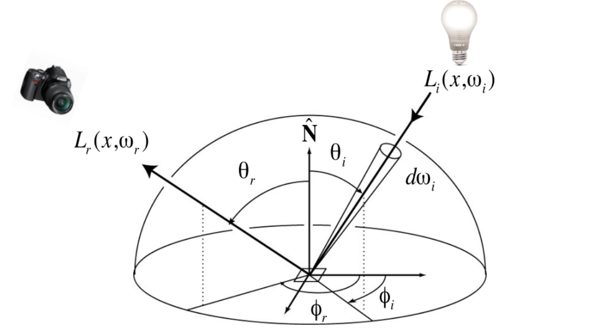
Where:

• $L _ {o}$ is the outgoing radiance
• $\pmb{p}$ is the rendering point
• $\pmb{\omega} _ {i}$ is the incident light direction
• $\pmb{\omega} _ {o}$ is the outgoing light direction
• $L _ {e}$ is the emissive radiance
• $\pmb{n}(\pmb{p})$ is the surface normal at point $\pmb{p}$
• ${\mathcal{H}^2(\pmb{n}(\pmb{p}))} $ is the hemisphere with normal $\pmb{n}(\pmb{p})$
• $f _ {r}$ is the bidirectional scattering distribution function (BRDF)
• $L _ {i}$ is the incoming radiance
• $\theta _ {\pmb{\omega} _ {i},\pmb{n}(\pmb{p})}$ is the angle between $\pmb{\omega} _ {i}$ and $\pmb{n}(\pmb{p})$.

The reflection equation is defined as: \(L _ {r}(\pmb{p},\pmb{\omega} _ {o})=\int _ {\mathcal{H}^2(\pmb{n}(\pmb{p}))} f _ {r}(\pmb{p},\pmb{\omega} _ {i},\pmb{\omega} _ {o})L_i(\pmb{p},\pmb{\omega} _ {i})\cos\theta _ {\pmb{\omega} _ {i},\pmb{n}(\pmb{p})}\mathbb{d}\pmb{\omega} _ {i}\tag{2}\) Therefore, the rendering equation can be rewritten as: \(L _ {o}(\pmb{p},\pmb{\omega} _ {o})=L _ {e}(\pmb{p},\pmb{\omega} _ {o})+L _ {r}(\pmb{p},\pmb{\omega} _ {o})\) As $L _ {e}(\pmb{p},\pmb{\omega} _ {o})$ represents the intensity of object’s self-emission and can be treated as a known quantity, we assume that no objects other than the light source emit light spontaneously. Therefore, we only need to focus on the reflected light intensity $L _ {r}(\pmb{p},\pmb{\omega} _ {o})$. This can be expressed as: \(L _ {o}(\pmb{p},\pmb{\omega} _ {o})=L _ {r}(\pmb{p},\pmb{\omega} _ {o})\tag{3}\) In equation (2), the reflected light $L _ {r}(\pmb{p},\pmb{\omega} _ {o})$ actually comes from two parts:

• Direct illumination from the light source, called direct light, denoted as $L _ {\text{dir}}(\pmb{p},\pmb{\omega} _ {o})$;
• Indirect illumination from other objects, called indirect light, denoted as $L _ {\text{indir}}(\pmb{p},\pmb{\omega} _ {o})$.

In the equation (4), $-\pmb{\omega} _ {i}$ is the outgoing direction for $L_{\text{dir}}$ and $L_{\text{indir}}$.

2.2 Direct Lighting

2.2.1 Lighting Equation for Light Sources

For the light source $L_e$, the outgoing light direction is $\pmb{\omega} _ {e,o}=-\pmb{\omega} _ {i}$.

The position $\pmb{p}$, outgoing direction $\pmb{\omega} _ {o}$, and incoming direction $\pmb{\omega} _ {i}$ can be determined by three points, as shown in the following figure:

Figure 2

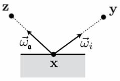
Note: In the figure, $\pmb{x}$ represents $\pmb{p}$, and $\pmb{y}$ represents $\pmb{p}^\prime$.

If we only integrate at the original lighting point $\pmb{p}$, we are sampling solid angles on a hemisphere, which leads to a lot of optical directions being wasted. Therefore, we should integrate directly over the region where the light source is located, i.e., the integration limit changes from a hemisphere to the surface area of the light source! \(L _ {\text{dir}}(\pmb{p},\pmb{\omega} _ {o})=L _ {\text{dir}}(\pmb{x}\to\pmb{z})=\int _ A f _ {r}(\pmb{y}\to \pmb{x}\to\pmb{z})L _ {e}(\pmb{y}\to\pmb{x})G(\pmb{x}\leftrightarrow\pmb{y})\mathbb{d}A(\pmb{y})\tag6\) Here, the integration domain $A$ includes all surfaces in the scene, but only at the position of the light source $L _ {e}(\pmb{y}\to\pmb{x})\neq 0$.

By applying the Monte Carlo integration method, we get: \(L _ {\text{dir}}(\pmb{x}\to\pmb{z})=\sum _ {A(i,j)}\frac{ f _ {r}(\pmb{y}\to \pmb{x}\to\pmb{z})L _ {e}(\pmb{y}\to\pmb{x})G(\pmb{x}\leftrightarrow\pmb{y})}{p(i,j)}\tag7\) Where, $p(i,j)$ is a uniformly sampled point on the surface of the light source region $A$.

By changing variables in the integral using eq(5) and eq (6), we get:

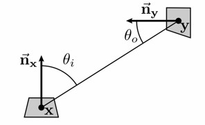
Where, $\theta _ {\pmb{y},\pmb{x}}$ represents the angle between the direction $\pmb{x}-\pmb{y}$ and the normal vector $\pmb{n}(\pmb{y})$ at point $\pmb{y}$. We introduce a geometric term to represent the “transport efficiency” between the two points:

Where, $V(\pmb{x}\leftrightarrow\pmb{y})$ is a visibility function, which is 1 if there is no occlusion between $\pmb{x}$ and $\pmb{y}$, and 0 otherwise. $G$ is a symmetric function, meaning that $G(\pmb{x}\leftrightarrow\pmb{y})=G(\pmb{y}\leftrightarrow\pmb{x})$.

If we denote the number of light sources in the scene as $N_e$, the set of light sources as ${L _ {e _ {i}}} _ {i=1}^{N _ {e}}$, and the corresponding regions as ${A(L _ {e _ {i}})} _ {i=1}^{N _ {e}}$, then we can write the equation as: \(\begin{aligned} L _ {\text{dir}}(\pmb{x}\to\pmb{z})&=\sum _ {k=1}^{N _ {e}}\int _ {A(L _ {e _ {k}})} f _ {r}(\pmb{y}\to\pmb{x}\to\pmb{z})L _ {e}(\pmb{y}\to\pmb{x})G(\pmb{x}\to\pmb{y})\mathbb{d}A(\pmb{y})\\ &=\sum _ {i=k}^{N _ {e}}\sum_ {A_k(i,j)} \frac{f _ {r}(\pmb{y}\to\pmb{x}\to\pmb{z})L _ {e}(\pmb{y}\to\pmb{x})G(\pmb{x}\to\pmb{y})}{p_k(i,j)} \end{aligned}\tag8\)

2.2.2 Importance Sampling for Environment Map

Monte Carlo Importance Sampling

In addition to being emitted from the light sources we specify, direct lighting can also come from ambient illumination in the surroundings. When sampling the environment map, if we uniformly sample all regions of the environment map, we will lose a lot of information from regions with high radiance. Therefore, we should use Monte Carlo importance sampling to focus on sampling regions with higher radiance, as shown in the figure below.

Figure 3: MC Important Sampling

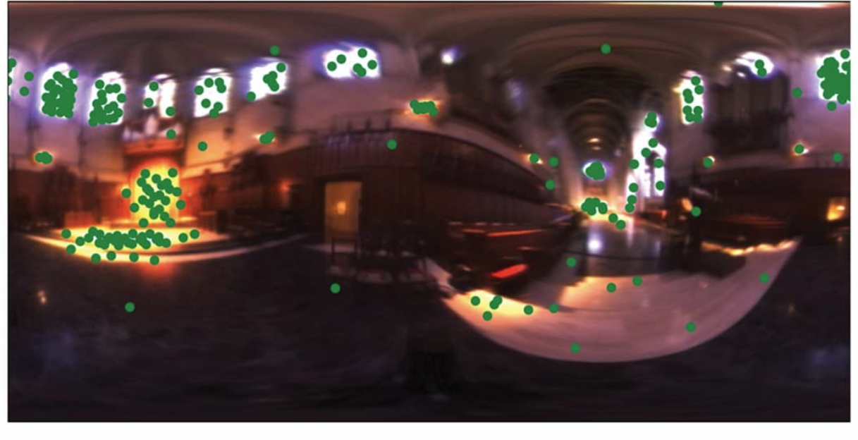
The so-called importance sampling means that the selected sampling probability density approximately conforms to the distribution to be sampled. For a given environment map, if the sampling is at pixel point $\pmb{y}=(i,j)$, the probability of that point is denoted as $p _ {img}(i,j)$. \(p_{img}(i,j)=\frac{L_e(i,j)}{\sum_{k,l}L_e(k,l)}\tag9\) The relevant probability relationships are as follows:

According to Figure 2 and the correspondence between environment map, we have:

where:

• $i \in [0, w]$，$w$ is the image width.
• $j\in[0,h]$，$h$ is the image height.

• $u,v\in[0,1]$，and $u=i/w$, $v=j/h$.

• $\theta\in[0,\pi]$，$\theta=\pi(1-v)$
• $\phi\in[0,2\pi]$，$\phi=2\pi u$
• $\pmb{\omega} _ i=(\sin\theta\sin\phi,\cos\theta,\sin\theta\cos\phi)$

So that: \(p(\pmb{\omega} _ {i})=\frac{wh}{2\pi^2\sin\theta}p _ {\text{img}}(i,j)\tag{10}\) At this point, eq (6) can be rewritten as: \(\begin{aligned} L _ {\text{dir}}(\pmb{p},\pmb{\omega} _ {o})&=\int _ A f _ {r}(\pmb{y}\to \pmb{x}\to\pmb{z})L _ {e}(\pmb{y}\to\pmb{x})G(\pmb{x}\leftrightarrow\pmb{y})\mathbb{d}A(\pmb{y}) \\&=\int _ {\mathcal{H}^2}\frac{ f _ {r}(\pmb{p},\pmb{\omega} _ {i},\pmb{\omega} _ {o})L_i(\pmb{p},\pmb{\omega} _ {i})\cos\theta _ {\pmb{\omega} _ {i},\pmb{n}(\pmb{p})}}{p(\pmb{\omega} _ {i})}\times p(\pmb{\omega} _ {i})\mathbb{d}\pmb{\omega} _ {i} \\&=\int _ {I}\frac{ f _ {r}(\pmb{p},\pmb{\omega} _ {i},\pmb{\omega} _ {o})L_e(\pmb{p},\pmb{\omega} _ {i})\cos\theta _ {\pmb{\omega} _ {i},\pmb{n}(\pmb{p})}}{p(\pmb{\omega} _ {i})}\times p _ {\text{img}}(i,j)\mathbb{d}i\mathbb{d}j \\&=\sum_{I_{i,j}}\frac{ f _ {r}(\pmb{p},\pmb{\omega} _ {i},\pmb{\omega} _ {o})L_e(\pmb{p},\pmb{\omega} _ {i})\cos\theta _ {\pmb{\omega} _ {i},\pmb{n}(\pmb{p})}}{p _ {\text{img}}(i,j)}\times \frac{2\pi^2\sin\theta}{wh} \end{aligned}\tag{11}\) The summation is a discrete sampling based on the importance distribution $p_{img}(i,j)$ obtained by importance sampling.

Alias Method

If the size of the environment map is $m=width \times height=n\times n$ pixels, the average time complexity of obtaining a sample point using conventional discrete sampling is $O(m)$. The Alias Method can reduce the time complexity of discrete sampling to $O(1)$. The specific steps are as follows:

Initialize Table

1. Suppose the initial probability distribution table is $U(k=i * n + j)=p(i,j) * m$, alias table $K_k =k$, where $k\in[0,m)$, and initialize two queues A and B to store the node numbers whose $U_k$ are less than 1 and greater than 1, respectively.

2. Pop a value $a=A.pop(), b=B.pop()$ from A and B queues, respectively.

3. Modify the probability distribution table: $U(b) = U(b) - (1 - U(a))$; modify the alias table: $K_k=b$.

4. If $U(b)<1$, add the element b to the A queue: $A.push(b)$

   If $U(b)>1$, add the element b to the B queue: $B.pushback(b)$

5. If A and B are both empty, end the process; otherwise, return to step 1.

Sample Operation

1. Generate two random numbers $\xi_1, \xi_2 \in [0, 1)$.

2. Let $k_1 = \lfloor m * \xi_1 \rfloor \in { 0, 1, 2, 3, …, m-1 }$.

3. If $\xi_2 \le U(k_1)$, then the sampled point is $(i, j) = (k_1%n, k_1/n)$.

   Otherwise, let $k_2 = K(k_1)$, and the sampled point is $(i, j) = (k_2%n, k_2/n)$.

The sampling time complexity of this algorithm is $O(1)$.

2.3 Indirect Lighting

2.3.1 Indirect Lighting Equation

In addition to computing direct lighting, “indirect lighting” must also be calculated. \(\begin{aligned} L _ {\text{indir}}(\pmb{p},\pmb{\omega} _ {o}) =\int _ {\mathcal{H}^2(\pmb{n}(\pmb{p}))}L _ {r}(\pmb{p},-\pmb{\omega} _ {i})f _ {r}(\pmb{p},\pmb{\omega} _ {i},\pmb{\omega} _ {o})\cos\theta\mathbb{d}\pmb{\omega} _ {i} \end{aligned}\tag{12}\)

Figure 4: Indirect Light

If we look back at equation 4, we will find that indirect lighting requires recursion!

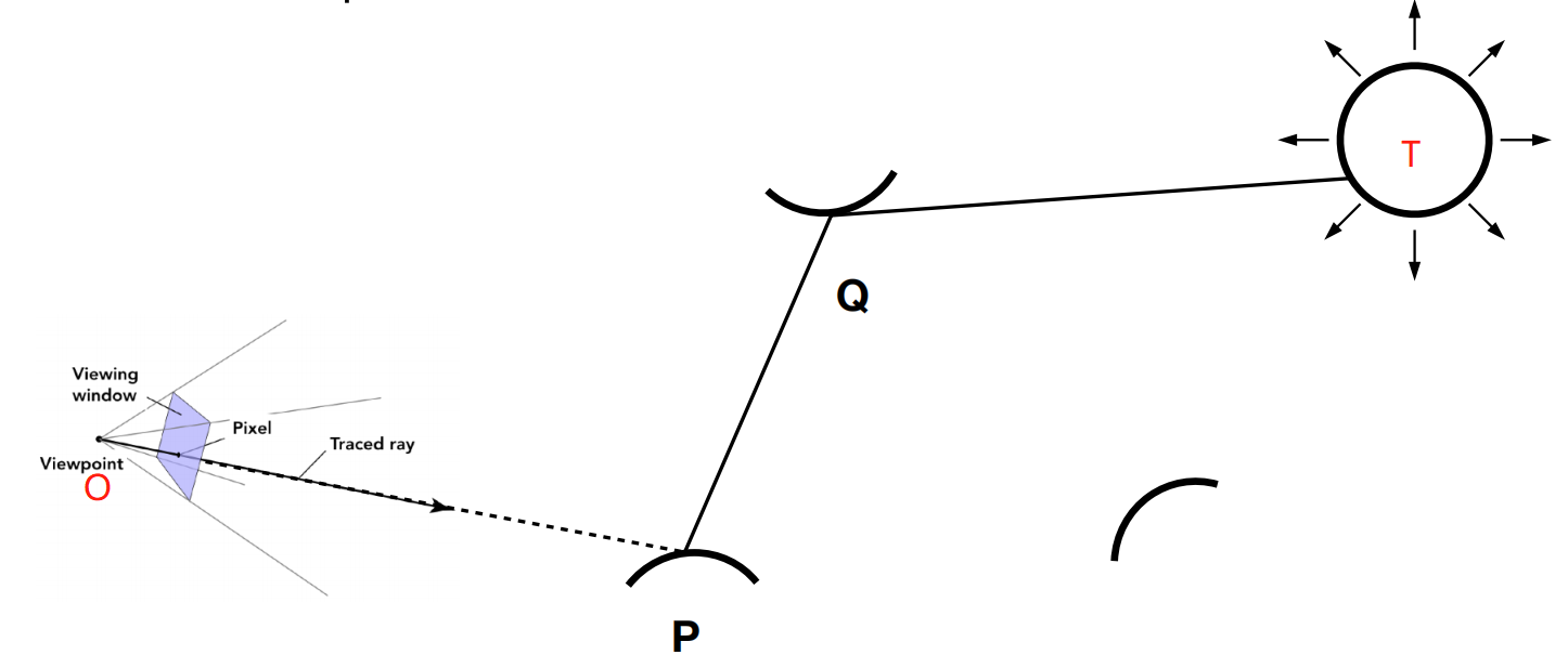
Assume that the camera is located at point O and the light source is at point T. We want to calculate the radiance of point P projected onto point O. We perform Path Tracing along the OPQ path:

• If no object is encountered, the recursion ends, and $L_o=L_r=L_{\text{dir}}$.
• If an object is encountered, we can regard Q as the light source. Then, we solve the first rendering equation for the OPQ segment. The incident radiance Li(p,ωi) at point P in the integrand of the equation is unknown, but this incident radiance Li at point P is also the outgoing radiance Lo at point Q. We can then solve the second rendering equation along the PQT path. We keep recursing until we encounter the environment or the light source.

2.3.2 The exponential explosion problem

1. As the number of bounces increases, the number of rays traced grows exponentially with N, the number of samples taken for each incoming direction. As a result, the recursion stack grows exponentially with the increase in recursion depth.

   Solution: The recursion explosion problem only occurs when N > 1. To avoid it, we only choose one incoming direction at random instead of N directions.

2. In the natural world, light bounces an infinite number of times, but setting an upper limit on the number of bounces will inevitably result in a loss of energy. So how can we avoid infinite recursion and energy loss?

   Solution: Russian Roulette (RR)

   • Our goal is to calculate the shading result of a shading point, i.e., the Lo in the camera direction.
   • Assume we manually set a probability P (0 < P < 1). We emit another ray with a probability of P and return the shading result of Lo/P. We do not emit another ray with a probability of 1 - P and return 0.
   • Finally, the expected value of the discrete random variable is calculated as: $E = P \times (Lo / P) + (1 - P) \times 0$.

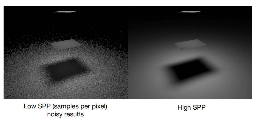
3. Since we only randomly sample one incoming direction, there may be a lot of noise. Some shading points may not hit the light source or other objects, even if the random incoming direction is sampled and calculated.

   Solution: Increase the samples per pixel (SPP) by tracing more paths per pixel and averaging them. Therefore, by tracing enough paths, there is a greater chance of hitting a valid light source or object, resulting in a closer approximation to the correct shading.

Figure 5: Compare spp

2.4 Algorithm

So far, we have obtained all the algorithms for solving equation 1, in pseudo-code form as follows:

Shade(p,wo):
	// 1、Direct illumination from light sources and ambient light.
    Uniformly sampling a point on the surface of the light source: x';   
	shoot a ray form p to x';
	L_dir = 0.0;	
	if (the ray is not blocked in the middle)
        if (the ray from source light)
			L_dir += L_e * f_r * cosθ * cosθ' / |x' - p|^2 / pdf_light;
    	else if(the ray from environment backgroud)
            L_dir += L_e * f_r * cosθ / pdf_env * (2*pi*2pi*sinθ)/(w*h)
	//2、Indirect illumination from other objects.
	L_indir = 0.0;
	Test Russian Roulette with probability P_RR;
	Uniformly sample the hemisphere toward wi;  
	Trace a ray r(p,wi);
	if (ray r hit a non-emitting object at q)
	    L_indir = shade(q, -wi) * f_r * cosθ / pdf_hemi / P_RR; 
    return L_dir + L_indir;

3 Result

3.1 low SPP

We simulate at low number of samples per pixel (SPP = 4).

3.1.1 Direct Lighting Only

First, consider only the direct lighting model \(L_o=L_{dir}\)

Figure 6: Only direct light

Result analysis: The effect of adding only direct lighting is not good for high reflectivity metal spheres, but it can already display the image basically.

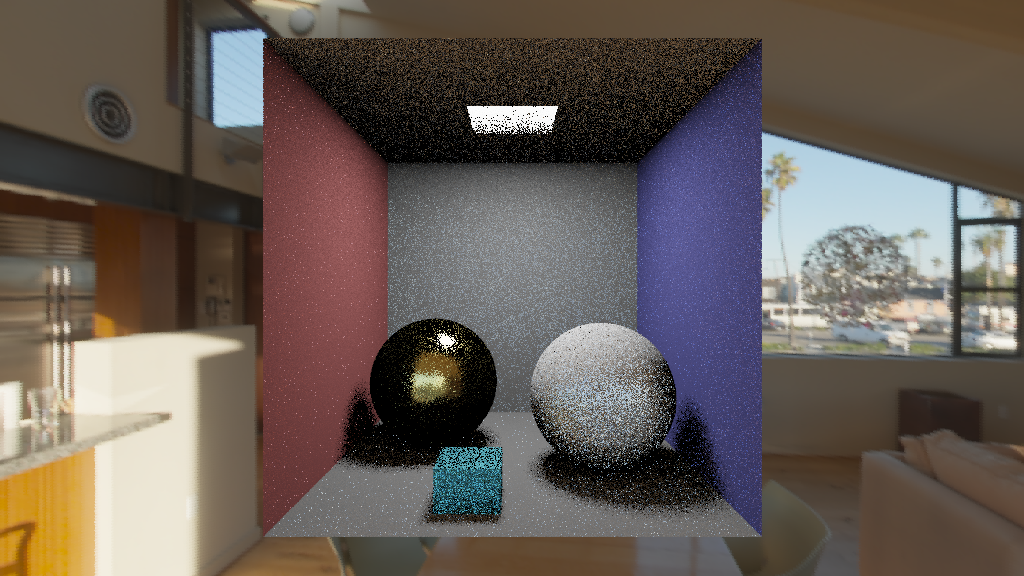
3.1.2 Global Illumination

Now we add indirect lighting, which means \(L_o=L_{\text{dir}}+L_{\text{indir}}\)

Figure 7: Global Illumination

Result Analysis: By adding indirect illumination, the metal sphere looks more realistic in the global illumination model and can clearly reflect patterns of other objects.

3.1.3 Monte Carlo Importance Sampling

Let’s consider importance sampling for the environmental light.

Figure 8: Global Illumination by important sampling

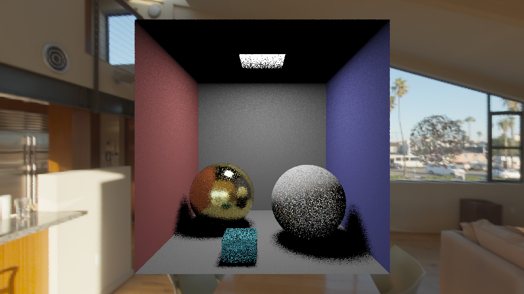
Results analysis: When importance sampling is applied to environmental lighting, the noise in the image is reduced and the shadows in the image are better displayed.

3.2 High SPP

Finally, we increase the number of SPP to 1024 and display the results.

Figure 9:Global Illumination with high spp

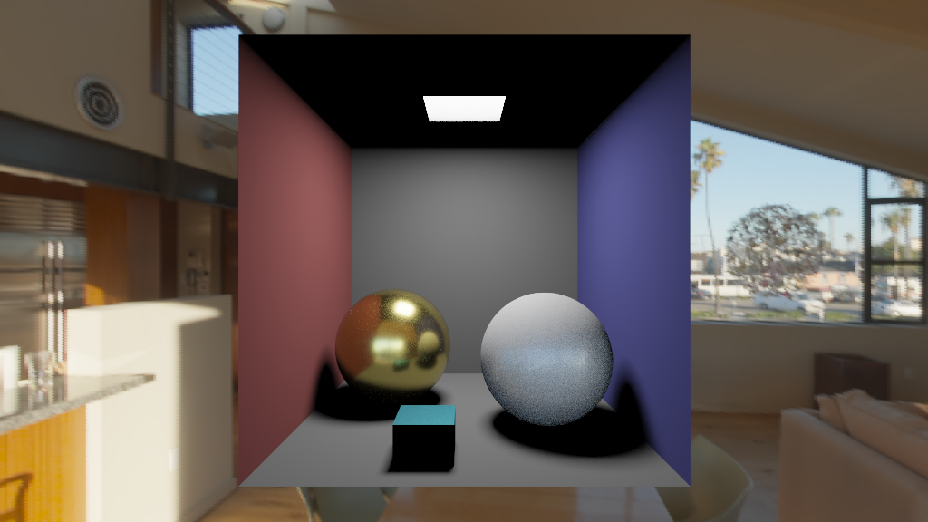
Result Analysis: With an increasing number of optical tracks being tracked, the scene has become very realistic, successfully rendering the image.

4 Summary

This article first analyzes the principles of the rendering equation and provides a reasonable decomposition of the rendering equation.

Then, we introduce how to use the Monte Carlo integration method for sampling, namely, the method of directly sampling the illumination and importance sampling by varying the sampling regions, and improves the sampling efficiency with the help of the Alias algorithm. The experimental results show that importance sampling has a good effect on improving image quality.

Next, the article elaborates on the method of recursively solving indirect illumination and proposes a series of methods to prevent the problem of exponential explosion.

Finally, after increasing the number of samples for each pixel, the image can successfully render the results.

5. Reference

[1] Code Framework