Seamlessly blend the image into the environment.

If you want to view the source code, you can search for them in my GitHub repository.

中文版本可以参见这个链接 click here

1 Abstract

Implementing image boundary determination based on the scan-line algorithm. And using a general interpolation mechanism based on solving the Poisson equation allows for seamless import of opaque and transparent source image regions into the target region.

Keywords: Interactive image editing, scanning line algorithm, Poisson equation

2 Target

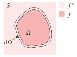
As shown in the figure, $f$ is the image to be blended with the domain defined in $\Omega$, and $f^*$ is the background image with the domain defined in $S$. The problem to be solved is to allow them to blend naturally. The so-called natural blending means that, while maintaining the original internal gradients of the image (minimizing the difference in gradients between the new and original images), the boundary values of the pasted image are the same as those of the new background image, in order to achieve a seamless paste effect.

3 Experiment

3.1 Polygon scan conversion algorithm

To better determine the boundary $\partial \Omega$ and the domain $\Omega$ to be solved, it is necessary to obtain a polygon interior mask through the scanline algorithm.

The sorted edge table method defines special data structures for the edge table ET and the active edge table AET, avoiding the need for intersection calculations.

Active Edge Table (AET）

This table stores the edges that intersect with the current scanline. Before leaving one scanline and entering the next one, the edges in the table that do not intersect with the next scanline are removed, and the edges that intersect with the next scanline but are not in the table are added to the table. The edges in the active edge table (AET) are always sorted in increasing order of their x-coordinates, because when filling the polygon, it is necessary to determine whether the algorithm is entering or exiting the interior of the polygon based on this order.

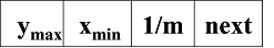
• ymax: The y-coordinate value of the highest scanline that the edge intersects.
• x: The coordinate of the intersection point between the current scanline and the edge.
• Δx:The increment of x from the current scanline to the next scanline.
• next: A pointer to the next edge.

Edge Table (ET)

(1) Before filling a polygon, it is necessary to first create an edge table to store information about the polygon’s edges. The edge table is a type of adjacency list. The entries in the edge table (ET) are sorted in increasing order of their y-coordinates, and the “bucket” under each entry is sorted in increasing order of their x-coordinates. The content of each item in the “bucket” is:

• The maximum y-coordinate (ymax) of the edge’s other endpoint.
• The x-coordinate (xmin) of the endpoint corresponding to the smaller y-coordinate.
• The reciprocal of the slope (1/m).
• A pointer (next) to the next edge.

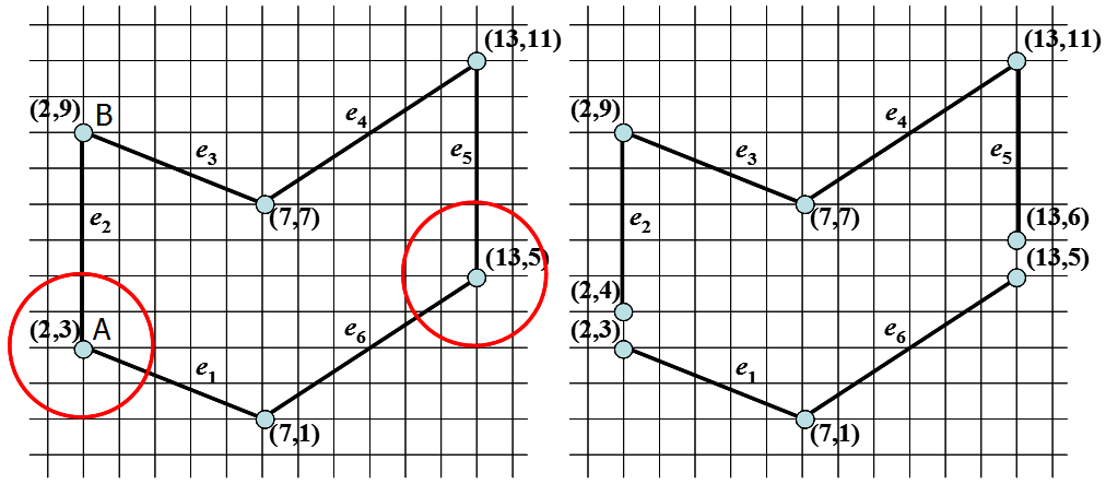
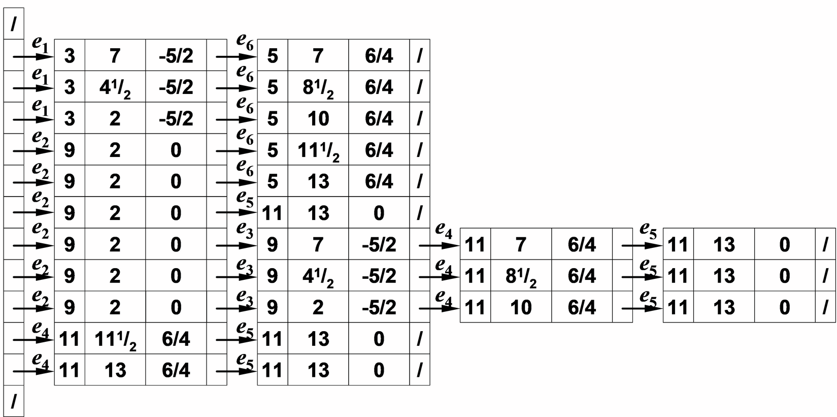
(2) Note: When creating the edge table, if a vertex appears to be a local maximum or minimum (e.g., point B in the figure below), it is treated as two separate points; otherwise, it is treated as a single point. In practice, local maximum or minimum vertices do not need to be processed, while other vertices should be moved inward along the edge direction by one unit.

The reason is as follows: For example, in the figure below, for point B, no extra processing is needed because when the scanline is at y=9, both e2 and e3 will be included in the AET. That is, point B will appear twice in the current AET, and when filling, it will enter and exit at that point, avoiding any filling errors. However, for point A, if it is not moved inward, when the scanline is at y=3, both e1 and e2 will be included in the AET. Therefore, point A will also appear twice in the current AET, resulting in three points in the AET and causing an error in the filling of the polygon interior after the row y=3. In addition, the AET should always contain an even number of points. After moving inward, point A will only appear once in the current AET, and there will be an even number of points, resulting in correct filling.

（3）The established ET is shown below:

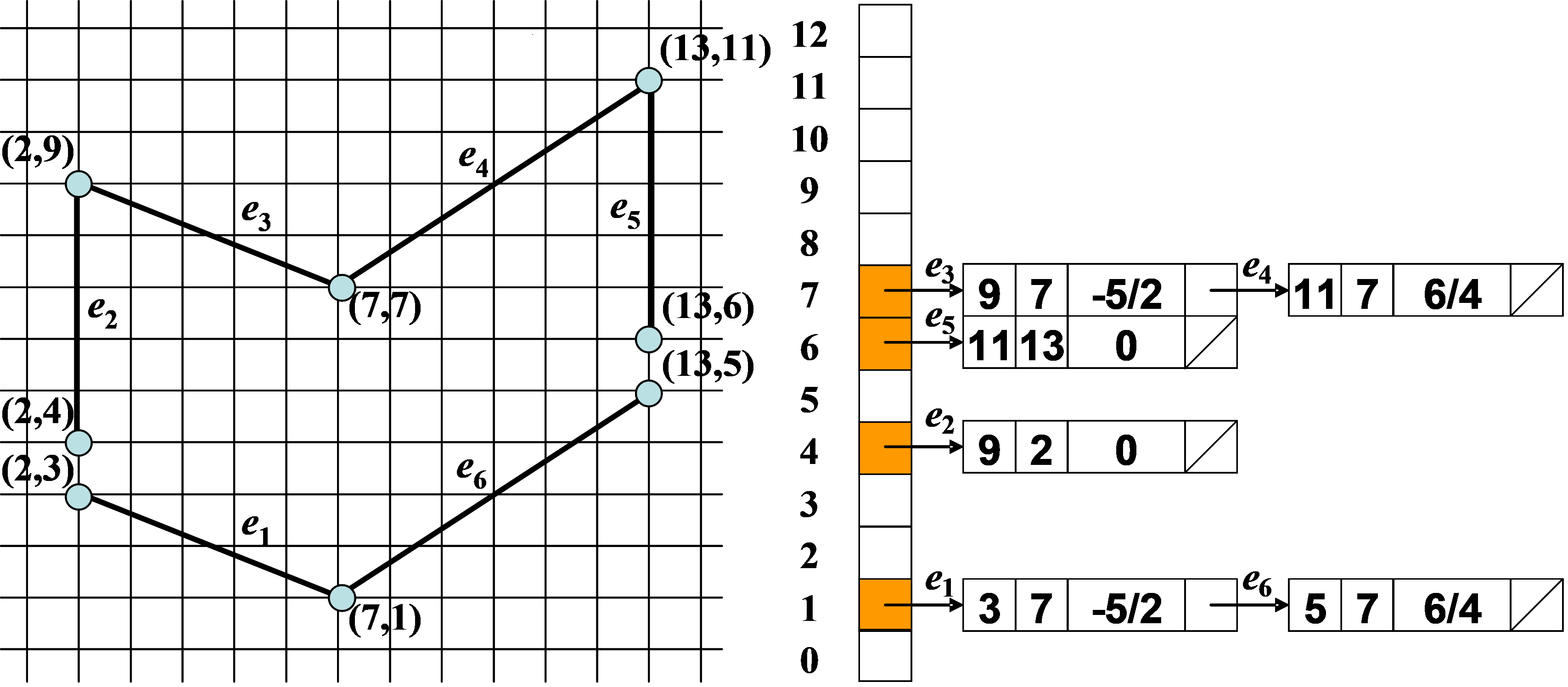
Note that e2 and e5 have been indented here, while e1, e3, and e4 have not.

Scanning process

Figure :Active Edge Table

Fill algorithm

void Polygonfill(EdgeTable ET,  COLORREF color)
{
    y = the minimum value of y coordinates among all the registered items in the edge table (ET).
    Initialize the active edge table (AET) as an empty table.
    while (there are still scan lines in the ET that have not been processed) // process each scan line in the ET
    {
    3.1 Merge all the "buckets" corresponding to the y coordinate in the ET into the AET table,
    sort the buckets in the AET table by increasing x coordinate.
    3.2 On the scan line y, perform fill using the color according to the x coordinates provided by the AET table.
    3.3 Clear all the items in the AET table that have y = ymax.
    3.4 For the remaining items in the AET table, replace x with x + 1/m.
    3.5 Since the previous step may have disrupted the increasing order of x coordinates in the AET table,
    re-sort the table by x coordinate. // for non-simple polygons
    3.6 Increment y by 1 and move on to the next scan line.
  	}
}

3.2 Image Fusion Algorithm

Mathematical Formulation

Mathematically, image fusion can be formulated as the solution to the optimization problem of embedding the new image $f(x,y)$ into a new background $f^ * (x,y)$ , given the original image $g(x,y)$, as follows:

\(\begin{equation} \min\limits_f \iint _\Omega |\nabla f-\nabla g |^2 \ \ \mathrm{with}\ f|_{\partial \Omega}=f^*|_{\partial \Omega} \end{equation}\tag1\) By using the variational method and applying the Euler-Lagrange equation, the problem can be transformed into a Poisson equation with Dirichlet boundary conditions: \(\begin{equation} \Delta f= \Delta g\ \mathrm{over}\ \Omega \ \ \mathrm{with}\ f|_{\partial \Omega}=f^*|_{\partial \Omega} \end{equation}\tag2\) If we let $\widetilde f = f - g$ and $(f^ * - g) = \varphi$, then the problem can be transformed into solving the boundary problem of Laplace’s equation:

Here, $f^*, g$ and $\varphi$ are known boundary conditions, while $\widetilde f$ is the function to be solved.

Numerical Equation

To perform numerical solutions, $\Delta f$ needs to be discretized using the finite difference method. Assuming a pixel spacing of $h=1$ for any point $\mathbf p=(i,j)$ in region $S$ with corresponding $f$ value denoted as $f_p$, the equation is as follows: \(\Delta f_p\approx\frac{4f(i,j)-f(i+1,j)-f(i-1,j)-f(i,j+1)-f(i,j-1)}{4h^2}\tag4\) For the sake of simplicity, let $N_p$ denote the four-connected neighborhood of each pixel $p$ in $S$. Let $\left<p,q\right>$ denote a pair of pixels such that $q \in N_p$, i.e., $q \in {(i+1,j),(i-1,j),(i,j+1),(i,j-1)}$. With this, we can obtain the numerical equation solution. \(\begin{equation} \mathrm{for}\ \mathrm{all}\ p\in \Omega,\ |N_p|\widetilde f_p-\sum\limits_{q\in N_p\cap \Omega} \widetilde f_q=\sum\limits_{q\in N_p\cap \partial \Omega}\varphi_p \end{equation}\tag5\)

Matrix Form Equation

Set $\widetilde f_{ij}=u_{ij},\varphi_p=\varphi_{ij}$, so that: \(4u_{i,j}-u_{i,j-1}-u_{i-1,j}-u_{i+1,j}-u_{i,j+1}=0\quad(i,j)\in \Omega\backslash\partial\Omega\tag6\)

If we take a rectangular region as an example, let \(\Omega={(i,j)|0\le i\le m,0\le j\le m}\) In this case, there are a total of $(m+1)\times (n+1)$ unknowns $u_{ij}$ in equations (5) and (6), and a total of $(m+1)\times (n+1)$ constraint conditions. These conditions are linearly independent, so the system is solvable.

For a more general boundary, the algorithm can be described as follows:

1. Initialization: Let there be a total of $N$ pixel points in $I=\Omega\backslash\partial\Omega$. Initialize a sparse $N\times N$ coefficient matrix coe_sparse_mat=0 and an N-dimensional unknown vector vec. Assume that the region $S$ has $n\times m$ pixel points and begin from the starting point.
2. Traverse each pixel point $(i,j)$ in the region $S$.
3. If $(i,j)\in I$, then index(i,j)=i*n+j
   • coe_sparse_mat[index(i,j)][index(i,j)]= 4
   • If a surrounding point $\mathbf q\in I$, then coe_sparse_mat(q)=-1
   • If a surrounding point $\mathbf q\in E=\partial\Omega$, then vec[index(q)]=$\varphi$[index(q)]
4. Solve the equation coe_sparse_mat * x=vec, where x(index(i,j)) = u(i,j).

// Step 1: Initialization
N = number of pixel points in D
coe_sparse_mat = sparse N x N matrix
vec = N-dimensional vector
n = number of pixels along x-axis in S
m = number of pixels along y-axis in S

// Step 2: Traverse pixel points in S
for i = 0 to m:
    for j = 0 to n:
    
        // Step 3: Check if pixel point is in D
        if (i, j) is in D:
            index = i * n + j
            coe_sparse_mat[index][index] = 4
            
            // Check surrounding points in Interior
            for each surrounding point q:
                if q is in D:
                    coe_sparse_mat[index][index(q)] = -1
                elif q is in E://if q in edge
                    vec[index(q)] = phi[index(q)]
                    
// Step 4: Solve equation coe_sparse_mat * x = vec
x = solve(coe_sparse_mat, vec)

The final solution is $\widetilde f_{ij}=u_{ij}$, and the pixel value of the resulting image is:

Where $g(i,j)$ is the pixel value of the original image, and $\widetilde f(i,j)$ is the value just obtained after solving.

4 Result

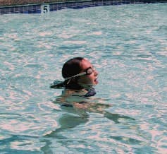
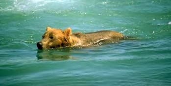
There is a girl happily swimming in the swimming pool, while a bear is swimming in another river. They are in different bodies of water, as shown in the following pictures.

Left:girl in the pool.Right: bear in the river

Now we put these two unlucky guys into the ocean. If we simply copy and paste, the following result would occur:

Simple Paste

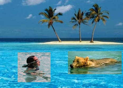
However, with the help of our Poisson fusion image algorithm, they can be more naturally integrated into the ocean：

Poisson Paste

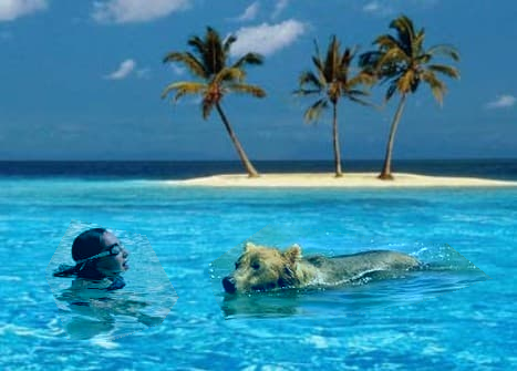
As you can see, the images match the surrounding environment more naturally after using our algorithm, but there is still room for improvement!

5. Reference

• Polygon Scan Conversion Algorithm
• Poisson Image Editing Algorithm
• Code Framework